One modeled scenario shows a plant shutdown causing zero lost sales because other plants and finished goods covered it; another shows a sole-source input cutoff eventually depleting finished goods and causing lost sales. This MIT capstone examines Tempur Sealy’s US network for Tempur-Pedic mattresses, while stressing that the findings are scenario analysis, not field results. The comparison can suggest that buffer location may matter as much as buffer volume.

The result challenges blanket stockpiling. Resilience spending should start with a specific uncovered failure, then test whether a proposed buffer lasts long enough for recovery to work. Inventory, sourcing, and logistics compete for funding but also interact. Finished goods may protect shipments while qualification protects replenishment. Transport matters only when the right product can reach the right destination on time.

Protection is measured in usable time

The modeled network tested plant shutdowns lasting three, six, and nine weeks across a full year. Other plants and finished goods buffers absorbed the output loss, with zero modeled lost sales. The disruption still depleted inventory and increased transfers. The network used its protection and paid for the recovery pattern.

A multi vendor input disruption behaved differently. Backup suppliers absorbed the interruption with little modeled change in service or cost. A sole source input cutoff eventually depleted finished goods and caused modeled lost sales and service failures.

The practical distinction is recovery time. A planner needs to know how long usable inventory lasts under actual demand and product mix, then compare that period with the time needed to qualify, produce, and move an alternative. A nominal stock level can look generous while offering little protection for important orders. Shared raw materials can preserve more mix options when production capacity is available.

The model compared equal percentage additions, not equal dollar investments. Adding 20% finished goods safety inventory produced about a 75% reduction in modeled lost sales. Adding 20% raw material inventory produced about a 53% reduction. Costs differ by mix, storage, expiry, obsolescence, capital, and handling, so these results do not mandate raising every buffer by 20%.

Alternate suppliers and transport routes can also share regional or infrastructure failures. A planning review should therefore check correlation explicitly rather than treating every backup as independent. The recommendation is to test whether proposed protections fail under the same disruption.

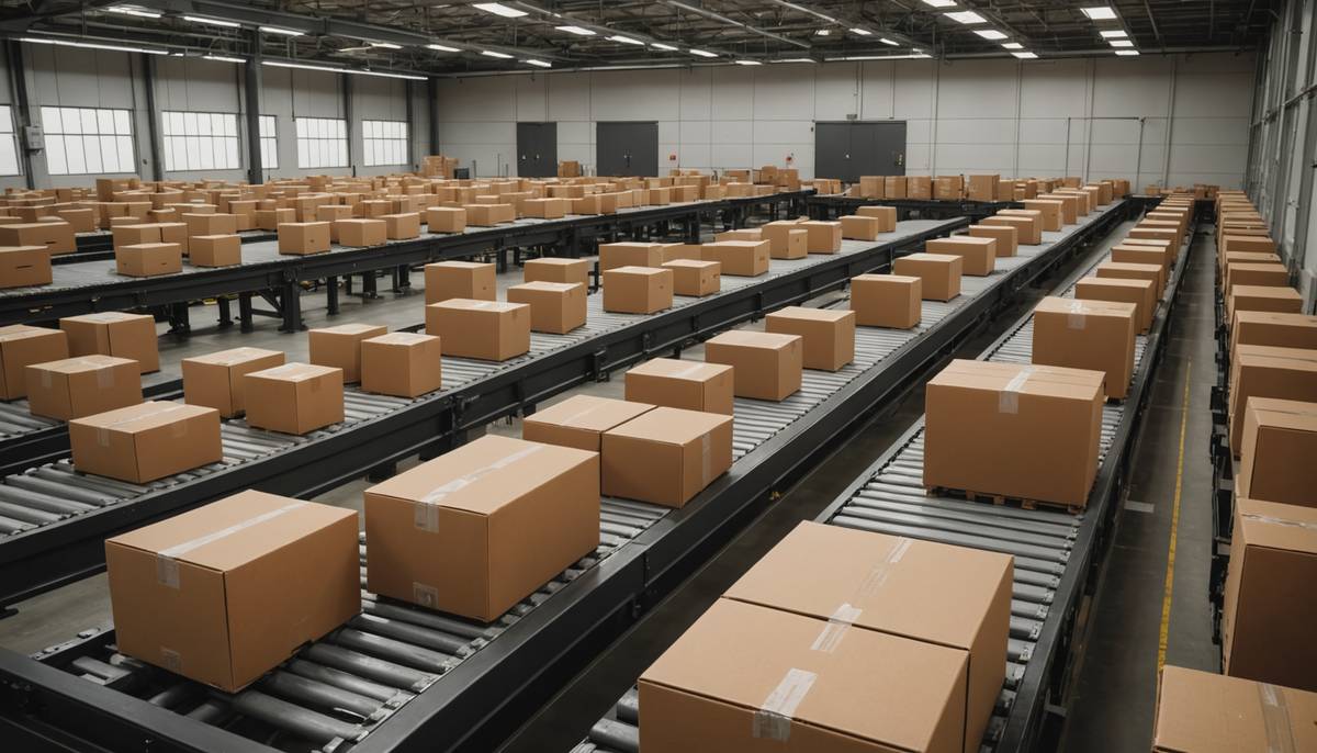
Compare packages around one product family

In an illustrative planning scenario, a planner responsible for delivery promises for one product family evaluates a sole source component, limited finished goods storage, and constrained transport lanes. The planner has one annual resilience budget. The question is which uncovered failure deserves the next dollar.

Compare three packages sized to the same annual budget: more finished goods inventory; a qualified alternate supplier with a capacity test; or smaller inventory paired with reserved logistics from an alternate origin. Hold demand, product mix, disruption, and recovery assumptions constant across packages. Then compare inventory coverage against recovery time, showing whether each budget buys protection before failure or faster replenishment afterward.

Start with a practical failure and recovery duration, then test usable inventory duration under the actual demand mix, qualified alternative capacity, and feasible transport under the same disruption and correlation assumptions. On a common evaluation horizon, value the residual lost orders at contribution margin and add recovery costs, annual carrying, storage, and obsolescence costs, plus one off qualification costs. Assess each lever together so the same saved orders are not counted twice across inventory, supplier, and logistics benefits. This makes the comparison reflect both service exposure and the full economic burden of resilience choices, including the time required to restore supply when alternatives are constrained.

Probabilities will rarely be precise enough for a confident ranking. Use ranges for disruption duration, qualification time, demand mix, capacity, and transport availability. Record the named assumption owner, its expiry date, and the review trigger. A package that remains preferable across reasonable ranges deserves more confidence than one that wins only under an optimistic assumption.

Make the allocation decision reviewable

The allocation may favor finished goods when customer promises are exposed and recovery is slow. It may favor shared raw materials when they preserve mix flexibility and production capacity can respond. It may favor supplier qualification when sole source exposure dominates. Logistics can strengthen these choices, yet it cannot replace missing product, capacity, or a qualified origin.

Review the decision when a sole source changes, an alternate loses capacity, demand mix shifts, storage economics deteriorate, a transport origin changes, or an assumption expires. Recalculate residual lost contribution margin, recovery costs, and ongoing carrying costs on the same horizon. Protection for the largest exposed family is not automatically the best allocation because marginal protection per dollar and total cost still matter.

In the next product family budget review, name the specific sole source failure being covered, fund the selected inventory, qualification, or logistics package, state its coverage period, assign an assumption owner, and set the trigger for reassessment. The decision should be revisited if the component cannot be restored within the stated period, the alternate fails its capacity test, or the demand mix and transport route change materially.